[ 岡山大学 | 理学部 | 地球科学科 | 地球および惑星大気科学研究室 ]
- 全部の問題を解かなければならないというものではありません.
- とばしてもよいと思う問題には「#」を付けています.
- 難しいと思う問題には「%」を付けています.
- かなり難しい問題も混ざっています.
- できる人はいろいろやってみてください.
- それ以外の人は,できる範囲でやってみてください.
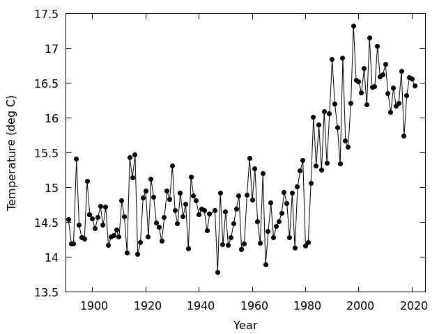
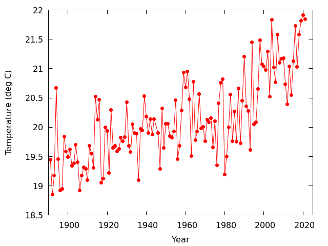
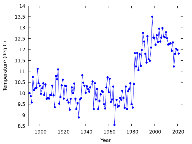
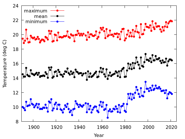
岡山の年平均気温の変化を見る
- 1891年から2021年の岡山の年平均気温,年平均日最高気温,年平均日最低気温
/home/atmos/ipesc/sample/amedas/Tave.dat
/home/atmos/ipesc/sample/amedas/Tmax.dat
/home/atmos/ipesc/sample/amedas/Tmin.dat
- まずはファイルの中身をみて,データの書式(データは何列あって,各列に何の数値が入っているのか)を確認する
- 図は見やすくなるように工夫する
- 点の種類を変えてみる,例えば pointtype を使う
- 点の大きさを変えてみる,例えば pointsize を使う
1891.01.01 - 1896.05.31 岡山城旧城郭内
1896.06.01 - 1949.04.15 岡山市内山下58番地
1949.04.16 - 1982.09.30 岡山市津島桑の木町1-16
1982.10.01 - 2015.03.04 岡山市桑田町1-36
2015.03.05 -            岡山市北区津島中2丁目
- 年平均日最低気温の図を見ると,1982年と1983年の間が不連続になっているとわかるが,これは観測露場を移転したことによるものであると考えられている
- 津島桑の木町は岡山大学農場の西,桑田町はイオンモール岡山の近く
- 中心市街地(桑田町)では,都市化の影響によって,郊外より高い気温が観測される
- 年平均気温の図でも,年平均日最低気温ほどではないが,1982年と1983年の間に不連続があるように見える
- 年平均日最高気温の図は,他の2つと違って不連続があるようには見えない
- 観測露場の変更は,日最低気温に大きな影響を及ぼしたが,日最高気温に対する影響はそれほどでもなかったらしい
- どの図をみても右上がりになっているので,温暖化していると思う人がいるかもしれないが,先に見たように観測露場移転の影響があるので,安直に温暖化していると結論することはできない
- また,ここ10年くらいは温暖化が止まっているように見えるが,これも2015年に観測露場が移転した影響を受けている可能性が高い
- 温暖化の評価は,移転の影響を取り除く必要があり,けっこう難しい
Skymonitor の稼働率を見る
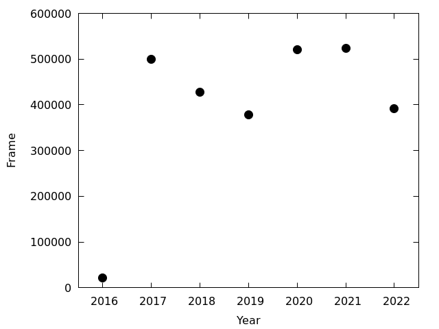
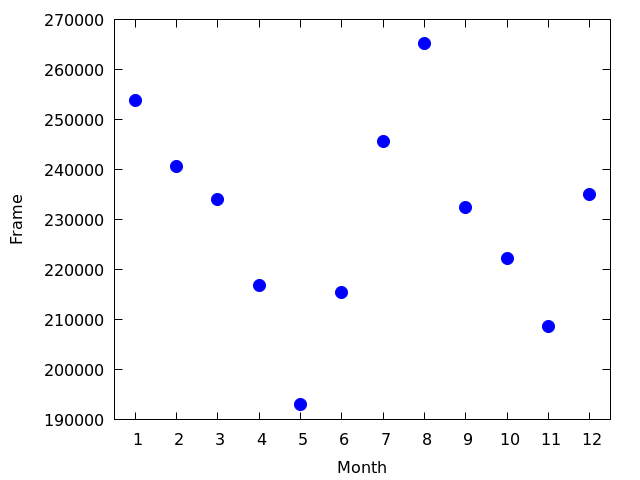
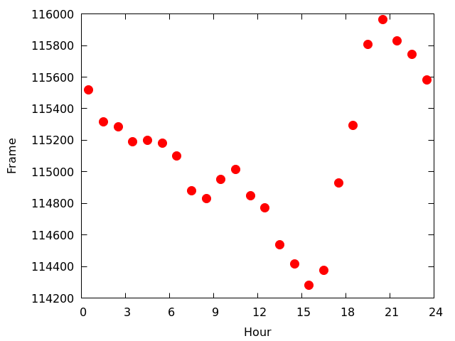
- 以下の3つのファイルには,Skymonitorが稼働し始めた2016年10月から2022年9月末までに撮影した写真について,各年に撮影した枚数,各月に撮影した枚数,各時間帯(0時台,1時台,...23時台)に撮影した枚数,が書かれている
/home/atmos/ipesc/sample/gnuplot/year.dat
/home/atmos/ipesc/sample/gnuplot/month.dat
/home/atmos/ipesc/sample/gnuplot/hour.dat
- 各年に撮影された枚数を図にして見る 図を見る
- 各月に撮影された枚数を図にして見る 図を見る
- 各時間帯に撮影された枚数を図にして見る 図を見る
- まずはファイルの中身をみて,データの書式(データは何列あって,各列に何の数値が入っているのか)を確認する
- 図は見やすくなるように工夫する
- 点の種類を変えてみる,例えば pointtype を使う
- 点の大きさを変えてみる,例えば pointsize を使う
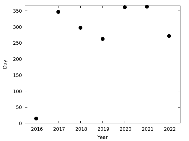
- 年ごとのデータ
- 1440 で割った値を表示してみる 図を見る
- まる1日稼働すると1440枚の写真が撮影される,すなわち1440で割ると稼働日数になる
- 2016年は定常運用前の試験運用中のため,稼働率が低い
- 2018年と2019年はカメラが不調で稼働率がちょっと低い
- 2019年の稼働率が低いのは,カメラを他のことに転用していた期間があるせいでもある
- 2022年の稼働率は10-12月を含んでいないので低くなっているが,9ヶ月分だと思うと稼働率は低くない
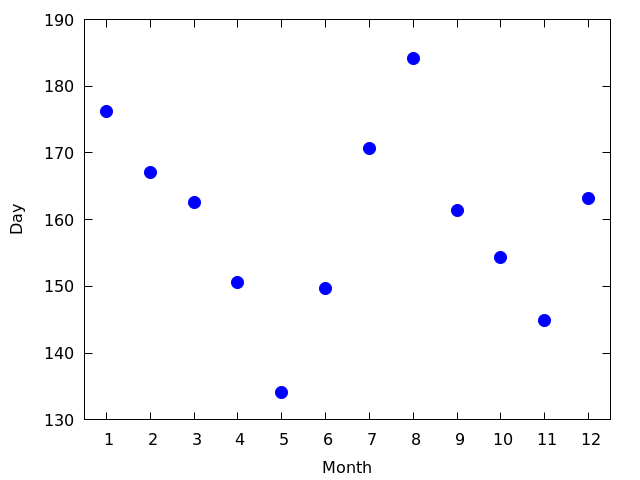
- 月ごとのデータ
- 1440 で割った値を表示してみる 図を見る
- まる1日稼働すると1440枚の写真が撮影される,すなわち1440で割ると稼働日数になる
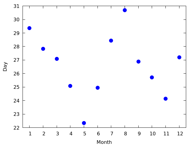
- 1440 で割ったものをさらに 6 で割る 図を見る
- 6 はスカイモニターが動き始めてからの(おおよそ)年数
- スカイモニターが定常運用を開始したのは2017年1月で,2016年のデータは少ない(ほとんどない)
- (おおよその)年数で割れば,(おおよその)1年あたりの稼働日数になる
- 2月と8月は欠測が少ない
- 8月は31日,2月はうるう年が1回あるので28.17日くらい
- 5月と6月の欠測が多いのは,2019年の5月と6月にスカイモニターの運用を停止していたため
- スカイモニターのカメラを他の用途で使っていた
- 5月と6月を 6 でなく 5 で割れば,2019年を除いたの5年間の稼働日数(1年あたり)になる
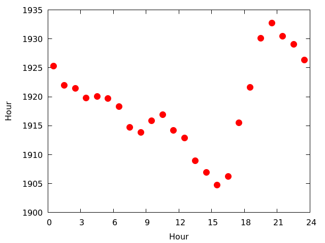
- 時間帯ごとのデータ
- 60 で割った値を表示してみる 図を見る
- まる1時間稼働すると60枚の写真が撮影される,すなわち60で割ると稼働時間数になる
- 各時間帯は1日につき1時間なので,稼働時間数=稼働日数である
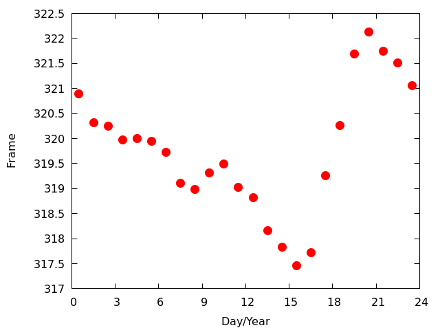
- 60 で割ったものをさらに 6 で割る 図を見る
- (おおよその)年数で割れば,(おおよその)1年あたりの稼働日数になる
- 最も稼働率が低いのは15時台(15:00-15:59),最も稼働率が高いのは20時台(20:00-20:59)
- 時間帯によって稼働率が異なる理由ははっきりとはわからないが,おそらく以下の2つで説明可能ではないかと思う
- スカイモニターが不具合を起こして停止する時間帯は特に決まっていない
- 不具合を修正して再稼働を始める時間は夕方であることが多い
文字の出現頻度を比べる
- 以下の6つのファイルには,4つのテキストにおいて各文字が使用された回数が書かれている
/home/atmos/ipesc/sample/text/char01.dat
/home/atmos/ipesc/sample/text/char02.dat
/home/atmos/ipesc/sample/text/char03.dat
/home/atmos/ipesc/sample/text/char04.dat
/home/atmos/ipesc/sample/text/char05.dat
/home/atmos/ipesc/sample/text/char06.dat
- 6つのテキストにおける文字の出現頻度を比較する図を作る
- まず6つのファイルの中身を見る
- ファイルの中身を見るには cat とか less とかを使う
- emacs で開いてもよい
- 図を作るとき,使いにくいものは無理に使わなくてもよい
- 1列目は数字じゃないので使いにくい
- 図にするだけなら0列目を使えばよい
- 6つのテキストは文字数が異なるので,使用回数そのままを図にしても,わかりやすい図にならない.文字数で規格化して図にするのがよい.
- ファイル datafile の2列目にある数字の和は,以下で計算することができる
$ awk '{print $2}' datafile | xargs | tr ' ' '+' | bc
- 文字の出現頻度からテキストを推定する
- 6つのテキストは
/home/atmos/ipesc/sample/text/Close_to_you.txt
/home/atmos/ipesc/sample/text/Hotel_Mauna_Kea.txt
/home/atmos/ipesc/sample/text/Lorem_ipsum.txt
/home/atmos/ipesc/sample/text/My_favorite_things.txt
/home/atmos/ipesc/sample/text/Potential_Vorticity.txt
/home/atmos/ipesc/sample/text/Pangram.txt
Lorenzアトラクタを描いてみる
- Lorenz方程式を数値積分した結果 /home/atmos/ipesc/sample/chaos/lorenz.dat
- データは 4 列で,左から t, x, y, z
- x-y 平面,x-z 平面,y-z 平面,などで図を描いてみる
- t-x 平面,t-y 平面,t-z 平面,などで図を描いてみる
- 初期値をちょっとだけ変えてLorenz方程式を積分した結果 /home/atmos/ipesc/sample/chaos/lorenz-dx.dat と比較してみる
- 点が大きいと重なってしまって見えにくくなるので,サイズを小さくしてみる.たとえば pointsize 0.1
- あるいは点で描くのをやめて線で描いてもいいかも
Edward N. Lorenzが大気の流れを表す方程式を簡略化して導いた連立方程式.
\begin{eqnarray}
\frac{dx}{dt} & = & P ( y - x ) \\
\frac{dy}{dt} & = & - y - x z + R x \\
\frac{dz}{dt} & = & x y - b z
\end{eqnarray}
決定論的な常微分方程式であるが,カオス的な振る舞いをする.
- 大雑把に分けて,x>0 でぐるぐるまわる場合と,x<0 でぐるぐるまわる場合,2通りあるのがわかる.
- x>0 でぐるぐるまわるのと,x<0 でぐるぐるまわる,この間の遷移に規則性があるように見えない(非周期性).
- 初期値がほんのちょっと違う場合,しばらく経つとまったく違う状態になってしまう(初期値鋭敏性).
- lorenz.dat と lorenz-dx.dat の1行目を比べれば,初期値にどれくらいの差があるか確認できる.
- 予測不可能性とも呼ばれる.ある期間より先の天気予報ができない原因.
gnuplot> splot '/home/atmos/ipesc/sample/chaos/lorenz.dat' using 2:3:4 with lines
とすると,xyz を3次元でプロットする.
図の上にカーソルを持っていって,クリックしたままカーソルを動かすと,視点を変えることができる.
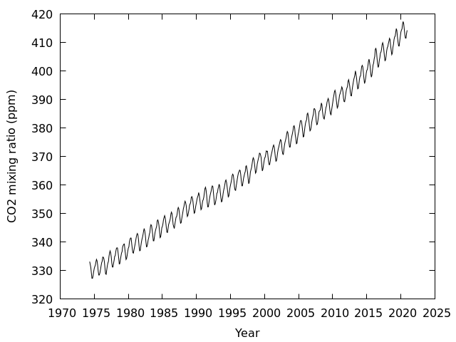
CO2濃度
- マウナロアで測定されたCO2濃度のデータ(ソース)
/home/atmos/ipesc/sample/co2/insitu.txt
- まずはデータを見る
- シェルで cat や less を使う
- 先頭から151行目まではデータについての説明が書いてある
- データの本体があるのは152行目から
- gnuplot は行頭が # で始まる行を注釈とみなして無視する
- 先頭から始まるデータの説明が書かれた部分について特別なことをしないでもよい
- CO2濃度は9列目,観測時刻を年で表した数値が8列目にあるので,時系列を表示するなら
gnuplot> plot '/home/atmos/ipesc/sample/co2/insitu.txt' using 8:9 with lines
- 欠測したもの(-999.99)は表示しないようにする
gnuplot> set datafile missing '-999.99'
gnuplot> plot '/home/atmos/ipesc/sample/co2/insitu.txt' using 8:9 with lines
図を見る
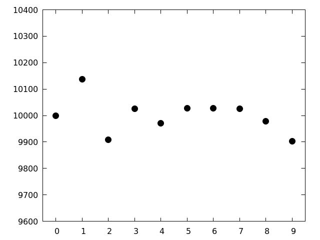
円周率に出てくる数字の出現頻度を見る. 図を見る
- 円周率100000桁に出てくる各数字の出現頻度は「シェルスクリプト練習問題2−6」で数えている
- 数えていないという人は,出現頻度を数えた結果が以下のファイルにあるので,それを使う
/home/atmos/ipesc/sample/number/pi.dat
- ランダムであるなら,各数字の出現確率は等しく 1 / 10 = 0.1
- 各数字の出現頻度の期待値は 100000 x 0.1 = 10000
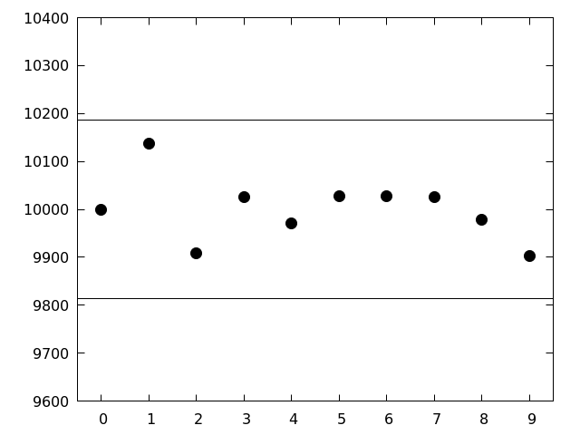
出現確率が 0.1 であった場合の出現頻度の95%信頼区間を重ね描きする. 図を見る
- n 回試行したとき,確率 p の事象が生じる回数の期待値は np
- n 回の試行で np が観測される,というわけではない
- サイコロを6回振ったときに1の目が出る回数は,1回のこともあれば,それ以外(0回だったり,2回だったり...)のこともある
- n が大きいとき,観測される回数の分布は np を中心とした正規分布になる
\[ \left[ n p - 1.96 \sqrt{ n p \left( 1 - p \right) } , n p + 1.96 \sqrt{ n p \left( 1 - p \right) } \right] \]
- 横軸に平行な直線は,数字そのままでプロットできる.例えば y=2 であれば
gnuplot> plot 2
- ある数字の出現する確率が p であるとき,その数字が n 個の数字の中に出現する数は95%の確率で以下の範囲にはいる
\[ \left[ n p - 1.96 \sqrt{ n p \left( 1 - p \right) } , n p + 1.96 \sqrt{ n p \left( 1 - p \right) } \right] \]
- いずれの数字も95%の範囲に入っているので,各数字の出現頻度はランダムである場合に予想されるばらつきの範囲内にあると言える
- 予想されるばらつきの範囲内にあるからといって,「ランダムである」と結論することはできない
- もし仮に95%信頼区間外の頻度が観測されていたとしても,それをもって「ランダムではない」ということにもならない
\begin{eqnarray}
1.64 \sigma & \ \ & 90\% \\
1.96 \sigma & \ \ & 95\% \\
2.58 \sigma & \ \ & 99\% \\
3.29 \sigma & \ \ & 99.9\%
\end{eqnarray}
各数字の出現確率を見る.
- 2列目を100000で割ったらよい,簡単にやるなら
using 1:($2/100000.0)
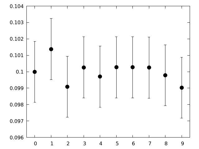
各数字の出現確率を区間推定し,出現確率と95%信頼区間を表示する. 図を見る
- n個の中にm個あったなら,その出現確率の点推定は m/n
- 95%信頼区間は,p = m/n として,
\[ \left[ p - 1.96 \sqrt{ \frac{ p ( 1 - p ) }{ n } } , \ p + 1.96 \sqrt{ \frac{ p ( 1 - p ) }{ n } } \right] \]
- using でデータを3列分指定し,with errorbars を使うと3列目を縦方向の誤差の大きさとして表示してくれる
using 1:2:3 with errorbars
- 区間の大きさを計算してデータの3列目として書き加えてもよいけど,2列目から計算するのが簡単だと思う
using 1:($2/100000.0):(1.96*(($2/100000.0)*(1.0-$2/100000.0)/100000.0)**(0.5)) with errorbars
n=100000.0
using 1:($2/n):(1.96*(($2/n)*(1.0-$2/n)/n)**(0.5)) with errorbars
- 区間推定の意味は,95%の確率でこの区間に入る,ということ
- 区間推定された範囲外にある確率は5%で,大きい可能性と小さい可能性がそれぞれ2.5%ずつ
- 信頼区間の幅は n の平方根に反比例する
- n を大きくすれば,出現確率をより狭い範囲で推定することができる
- 100桁だけとか1000桁だけとかで同じことをやってみて比べてみるといいかも
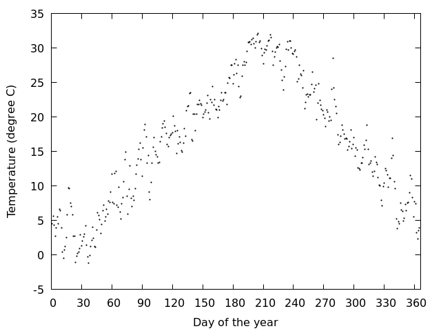
岡山で観測された日平均気温を1年分,図にしてみる 図を見る
アメダスのデータ(2018年)
/home/atmos/ipesc/sample/amedas/Okayama_Okayama_2018.csv
データは4列からなり,1列目から順番に,日付,日平均気温,日最高気温,日最低気温
gnuplot> set datafile separator ','
- 日付を扱うのはちょっと面倒なので,行番号(0列目)を使って表示する
- 1月1日を1にするなら,$0+1
gnuplot> plot 'Okayama_Okayama_2018.csv' using ($0+1):2
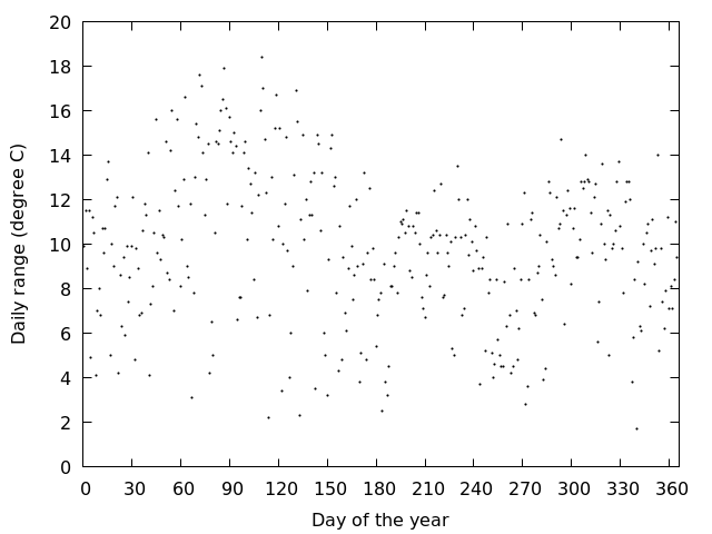
岡山で観測された気温の日較差を1年分,図にしてみる 図を見る
gnuplot> plot 'Okayama_Okayama_2018.csv' using 0:($3-$4)
- 日較差は季節によって大きくなったり小さくなったりしているように見える
- 日較差が季節に依って変わる理由を考えてみる
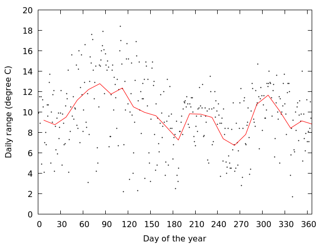
gnuplot> f(x)=(floor(x/a)+0.5)*a
gnuplot> a=15
gnuplot> plot 'Okayama_Okayama_2018.csv' u 0:($3-$4), '' using (f($0)):($3-$4) smooth unique
- 平均を求める期間を変えるには,a の値を変えればよい
gnuplot> a=5
gnuplot> plot 'Okayama_Okayama_2018.csv' u 0:($3-$4), '' u (f($0)):($3-$4) smooth unique
Last Updated: 2022/11/02, Since: 2019/11/07.
This page is generated by Makefile.rd2html.